Six LLM Serving Cost Surprises

Gangmuk Lim
Research MLSys Engineer
Related post
This is Part 3 of 5. Part 1 is here. Part 2 is here.
What I promise in this post
Heads up — this is a long and dense post. But it is full of interesting and (importantly) surprising observations about running LLM inference in the cloud, the kind that contradict the (wrong, sorry but wrong) intuition you have probably been carrying around. I promise the time you spend reading it will pay off. Grab a coffee.
Recap
In Part 1, four different oracles — vendor spec sheets, a roofline, Claude Opus 4.7, Gemini Pro — missed the measured throughput of a single fully-specified 70B deployment by 3–9×. In Part 2, I took one slice (Llama 70B on A10G, workload 2048-in / 512-out) and showed that across the nine feasible TP/PP configurations the throughput spread was 4.4× and the $/token spread was 7.5×, on the same model and the same workload. The highest-SM-utilization config was one of the worst on $/token.
That post answered "is the problem real?" This one answers "what does it look like when you push on every other axis at once?"
The claim this post will defend
Cost-optimal LLM serving is a joint optimization across six dimensions — model × workload shape × GPU type × parallelism (TP/PP) × engine settings × cloud topology — and the dimensions interact non-trivially. No rule, heuristic, or single-axis analysis recovers the optimum. Picking on any one axis and hoping the others align routinely costs 2-5× on $/token. The optimum has to be measured on the joint state, and the joint state drifts.
That is the one paragraph I want you to take away. The rest of the post is six concrete pieces of evidence for it, each one a heuristic-that-fails or a metric-that-lies, drawn from real measurements. If you only have ten minutes, read the takeaway section at the end — it lists the three things to do differently tomorrow morning.
What we measured
Three dense models — Qwen3-32B, Qwen2.5-72B-Instruct, Llama 70B — on AWS A10G (g5), L40S (g6e), A100-40GB (p4d), and A100-80GB (p4de) instances, across every feasible TP/PP combination we could launch, for workload shapes ranging from 128/128 to 16384/2048. vLLM, chunked prefill on, BF16 weights, gpu_memory_utilization=0.85. All $/M numbers below use AWS on-demand pricing in us-east-1. MoE models behave differently enough that they get their own post (Part 5).
There are six findings. None of them is derivable from reading the datasheet. Most of them contradict a heuristic somebody on your team is using right now.
Finding 1 — Throughput ≠ cost-efficiency
Throughput is not what you pay for. You pay for the GPU-hour. The metric you care about is $/M tokens — how many dollars this configuration spends per million tokens served. (This is the same unit every public LLM API uses on its pricing page.) Throughput is at best a proxy and at worst a distraction. A configuration that delivers 2× more throughput at 3× more cost is worse on $/token even though it wins any "throughput shootout."
To make the comparison fair, this figure fixes GPU count at 8 on L40S, then varies only the parallelism configuration. Same 8 L40S GPUs, four different ways of arranging them. Llama 70B BF16, 2048in / 512out:
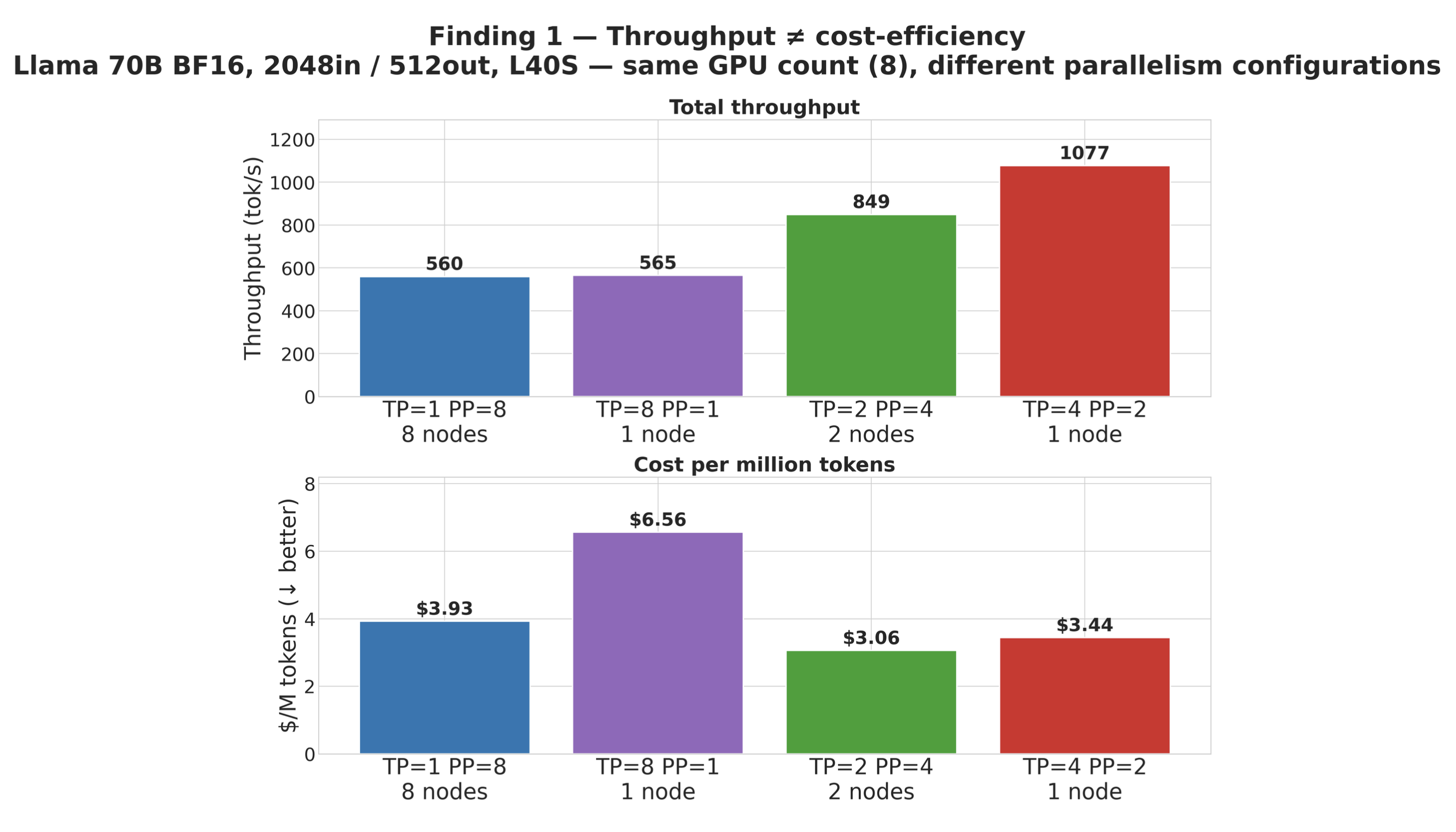 Figure 1. All feasible 8-GPU L40S configurations for Llama 70B at 2048in / 512out. Top: total throughput. Bottom: $/M tokens. Each configuration carries the same color across both panels.
Throughput spread: 1.92× (560 → 1077 tok/s). Cost spread: 2.15× ($3.06 → $6.56/M). Same model, same workload, same 8 GPUs. Four observations worth pulling out, because each one contradicts a heuristic you'd hear in a serving design review.
Observation 1 — TP=8 PP=1 and TP=1 PP=8 deliver almost the same throughput, but TP=1 PP=8 costs 40% less per token. 565 vs 560 tok/s, $6.56/M vs $3.93/M. Most people would call TP=8 PP=1 "the obvious choice" (8 GPUs in one box, no cross-node hop) and TP=1 PP=8 "the obviously bad choice" (8 separate machines, every layer crossing the network). Throughput says they're equivalent. Cost says the obviously-bad one wins.
The mechanism is per-GPU instance pricing, not parallelism:
| Instance | GPUs | $/hr | $/GPU/hr |
|---|---|---|---|
| g6e.2xlarge | 1 | $0.99 | $0.99 |
| g6e.12xlarge | 4 | $4.68 | $1.17 |
| g6e.48xlarge | 8 | $13.35 | $1.67 |
The 8-GPU box is 69% more expensive per GPU than the 1-GPU box on L40S. The "bigger instance is cheaper per unit" instinct people carry from CPU EC2 sizing does not apply here. Once throughput parity is established (TP=8 PP=1 ≈ TP=1 PP=8 in this case), the cheaper-per-GPU instance wins the dollar fight automatically.
Observation 2 — TP=2 PP=4 beats TP=8 PP=1 on both throughput AND cost. PP isn't always bad. 849 vs 565 tok/s (+50% throughput), $3.06 vs $6.56/M (-53% cost). This contradicts the textbook reflex that "pipeline parallelism is the parallelism of last resort because of pipeline bubble and inter-stage latency." That story is true for prefill of a single short request, but at sustained-batch throughput — which is what you pay for — the bubble amortizes across microbatches under continuous batching, and PP's per-step communication is cheaper than TP's all-reduce (a single activation send/recv between stages, not a per-layer all-reduce across the TP group). TP=2 PP=4 wins because: (a) TP=2 keeps the all-reduce small, (b) the 4 pipeline stages fit naturally on 4-GPU g6e.12xlarge boxes with TP within each node, (c) only PP boundaries cross node, and PP is point-to-point and small.
Observation 3 — TP=4 PP=2 is the intuitive winner. It's also not the cost winner. TP=4 PP=2 gives the highest throughput (1077 tok/s) and yes, that's exactly the config every "70B on L40S" recommendation we've seen on the internet lands on — including ep2. But TP=4 PP=2 costs $3.44/M while TP=2 PP=4 costs $3.06/M. For a 21% throughput sacrifice, you get 11% lower cost per token. If you optimized throughput and shipped TP=4 PP=2 to production — the "obvious" answer everyone agrees on — you would be quietly overpaying by ~12% on every token forever. Pipeline parallelism is not bad. Sometimes it's the cost winner even when it's not the throughput winner.
Observation 4 — three pieces of conventional wisdom violated by one chart. "TP > PP" — wrong: TP=2 PP=4 beats TP=8 PP=1 on cost by 53%. "Stay in one node" — wrong: the cheapest config (TP=2 PP=4) and the second-cheapest (TP=1 PP=8) both cross nodes; the most expensive one (TP=8 PP=1) is the single-node config. "Bigger instance is cheaper per unit" — wrong: g6e.48xlarge is 69% more expensive per GPU than g6e.2xlarge. None of these heuristics survive contact with the dollar bill.
The mechanism behind every observation is the same arithmetic identity: $/M = (price per hour) / (throughput per hour). Throughput optimization only touches the denominator. The numerator moves independently when you change instance size or topology. Optimize the ratio. Throughput is the wrong objective.
The 5× and 3× ratios make this sound like a sliding-scale efficiency problem. It is not. It is closer to a binary one. Picking the worst-half median costs you a third to a half of the tokens-per-dollar available at the same dollar cost. If you launch "something reasonable" without a sweep, that is what you are paying. Nobody bills you for the missing 40%. It just shows up at the end of the quarter as a cloud bill that is too big.
Finding 2 — SM% and HBM% both lie
In ep2 I said GPU SM utilization is not a useful north-star metric. People keep emailing me asking "okay then what about memory-bandwidth utilization, surely that one is honest." It is not.
Six configurations from the L40S 2048/512 sweep:
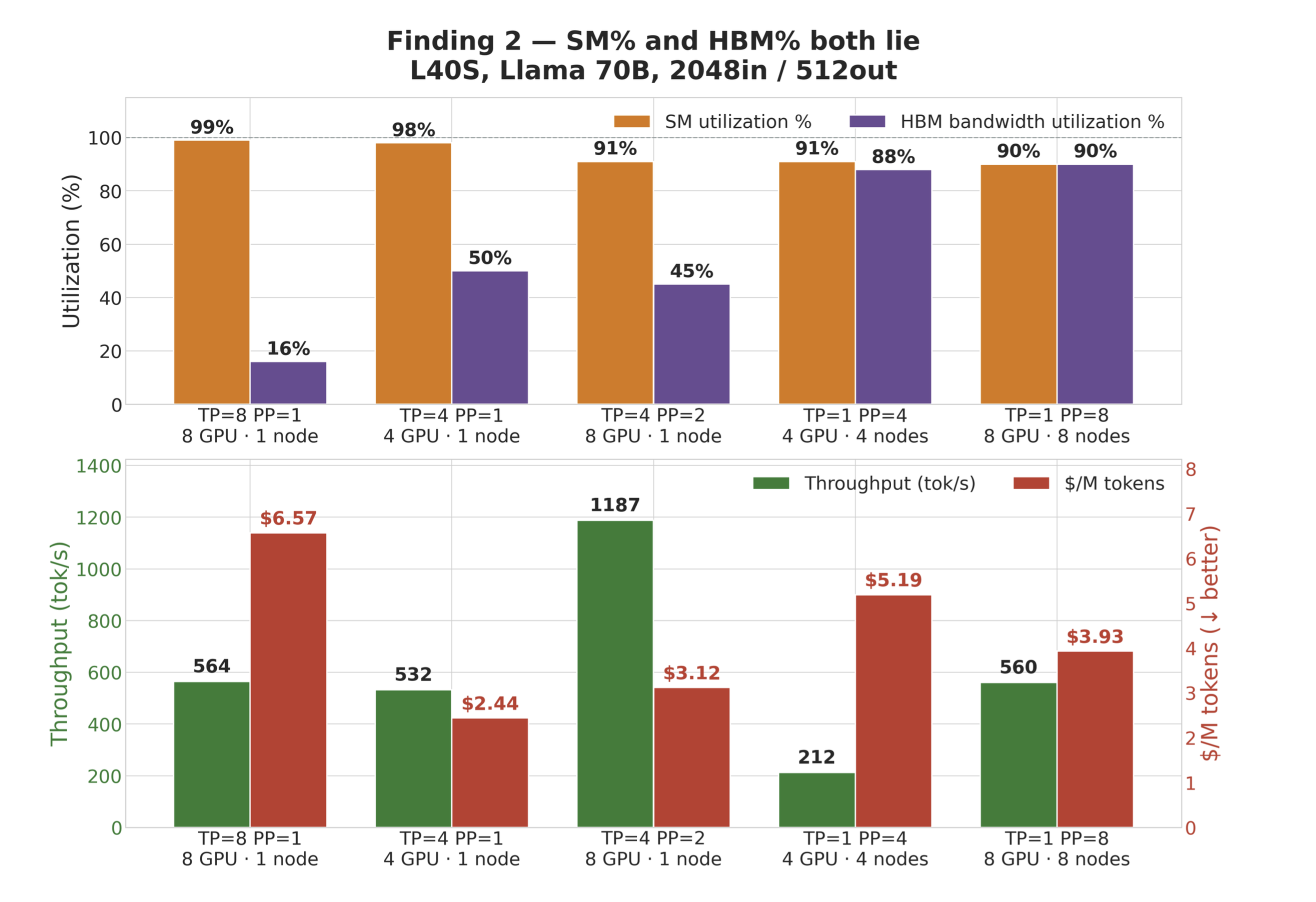 Figure 2. Top — SM utilization and HBM bandwidth utilization for six L40S configurations running Llama 70B at 2048-in / 512-out. Bottom — throughput (left axis, green) and $/M tokens (right axis, red) for the same configurations. Neither SM% nor HBM% tracks throughput or cost. The compute-saturated TP=8 PP=1 (99% SM) costs $6.57/M. The bandwidth-saturated TP=1 PP=K configurations (88–90% HBM) cost $5.19 and $3.93/M. The cost winner — TP=4 PP=1 g6e.12xlarge at $2.44/M — sits in the middle on both utilization metrics.
TP=8 PP=1 is compute-saturated. SMs running at 99%. Memory bus 84% idle. It is the worst $/M in the table. The compute is busy spinning on NCCL synchronization, not doing forward passes — and the reason NCCL is so expensive on this specific instance topology has its own deep mechanism. Part 4 dissects it; for now the observation is what matters.
TP=1 PP=4 and TP=1 PP=8 are the opposite pathology. Memory bandwidth pegged at 88-90% — closer to the decode-bound roofline than anything else in the whole sweep. Throughput is mediocre and $/M is bad. Each pipeline stage holds full layer weights and streams them through HBM cleanly; there is no NCCL, so the memory bus actually gets used. But the amount of compute per byte streamed is small because TP=1 cannot pack a big batch into one GPU.
The cost-optimal config (TP=4 PP=2 across 2× g6e.12xlarge) is in the middle on both metrics. SM% 91, MemBW% 45. Nothing about that pair of numbers tells you it is the cheapest.
A north-star metric you can optimize against has to point at the same configuration the dollar bill points at. SM%, MemBW%, KV-cache utilization, NCCL throughput — none of these do, individually or jointly. Optimize $/token directly.
Finding 3 — Adding GPUs doesn't always add work
Aggregate tok/s confounds "this config is good" with "this config has more GPUs." Normalize by GPU count and the picture gets honest very fast.
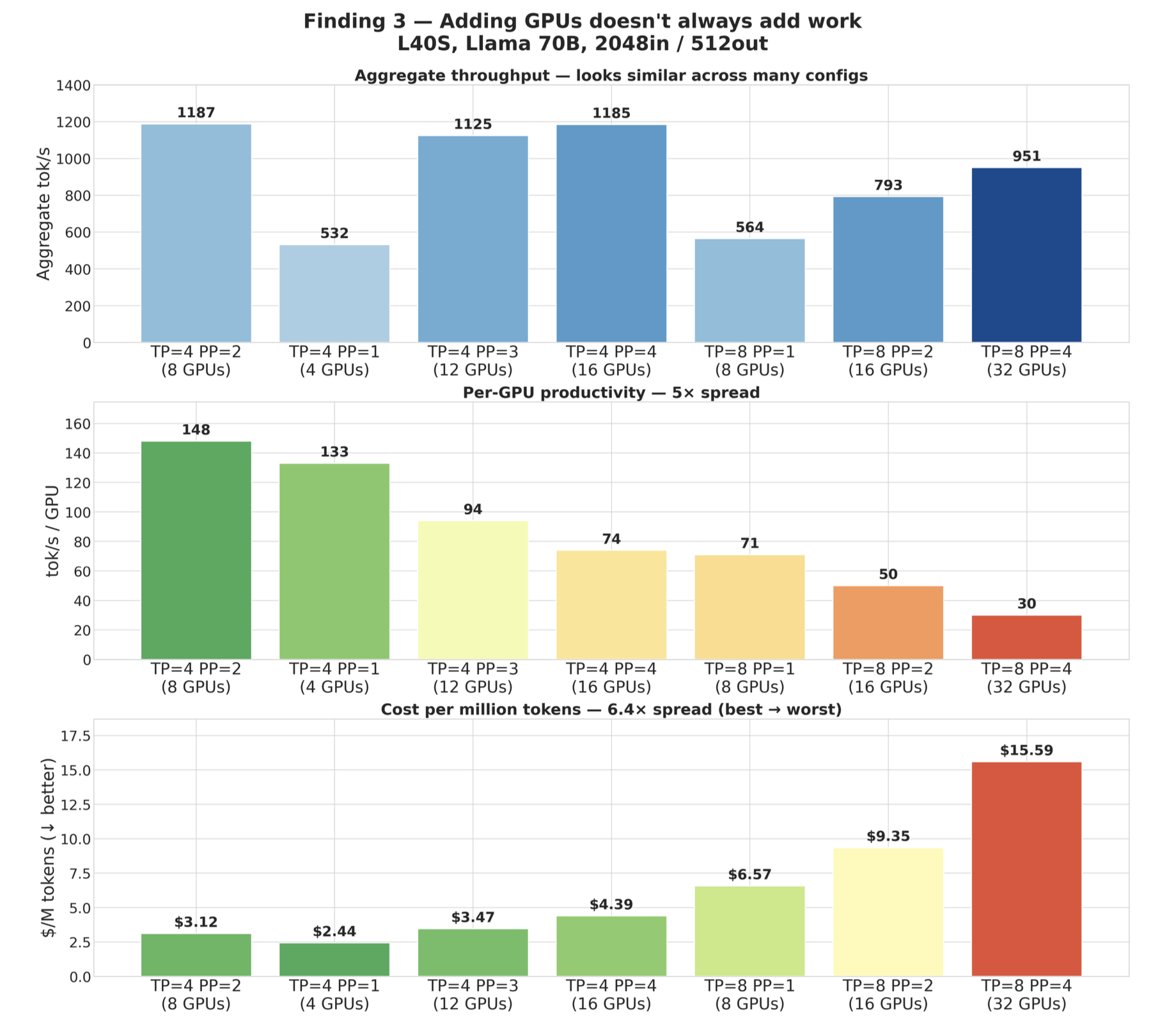 Figure 3. Three views of the same eight L40S configurations for Llama 70B at 2048-in / 512-out. Top — aggregate throughput (several configs look comparable). Middle — per-GPU throughput (a 5× spread reveals which configs waste marginal GPUs). Bottom — $/M tokens (a 6.4× spread translates the waste into cloud bill terms). TP=4 PP=1 on g6e.12xlarge wins on cost ($2.44/M) despite being the lowest aggregate throughput config that still uses ≥4 GPUs. TP=8 PP=4 on 4× g6e.48xlarge has competitive aggregate throughput (951 tok/s) but the worst cost ($15.59/M — 6.4× more than the winner).
Aggregate throughput says TP=4 PP=4 (1185 tok/s) and TP=4 PP=2 (1187 tok/s) are basically tied. Per-GPU productivity says TP=4 PP=4 is doing half the work per GPU that TP=4 PP=2 is. Same total throughput, double the silicon.
TP=8 PP=4 is the cleanest disaster. 32 GPUs, 30 tok/s per GPU. Each one of those L40Ss is doing 20% of what a TP=4 PP=2 L40S does. You are paying for 32 GPUs to get the work of about 6.5 of them.
This is the metric I would put in your dashboard. If tok/s/GPU drops below half of what you saw on the same model in a smaller config, the marginal GPU you added is not paying for itself.
Finding 4 — Workload picks the GPU
In Part 2 I showed that the optimal TP/PP changes when the workload changes. That is true and worth knowing. The bigger story is that even with the optimal config picked per workload, the cost floor moves enormously based on what your users type — and the cost-optimal GPU shifts.
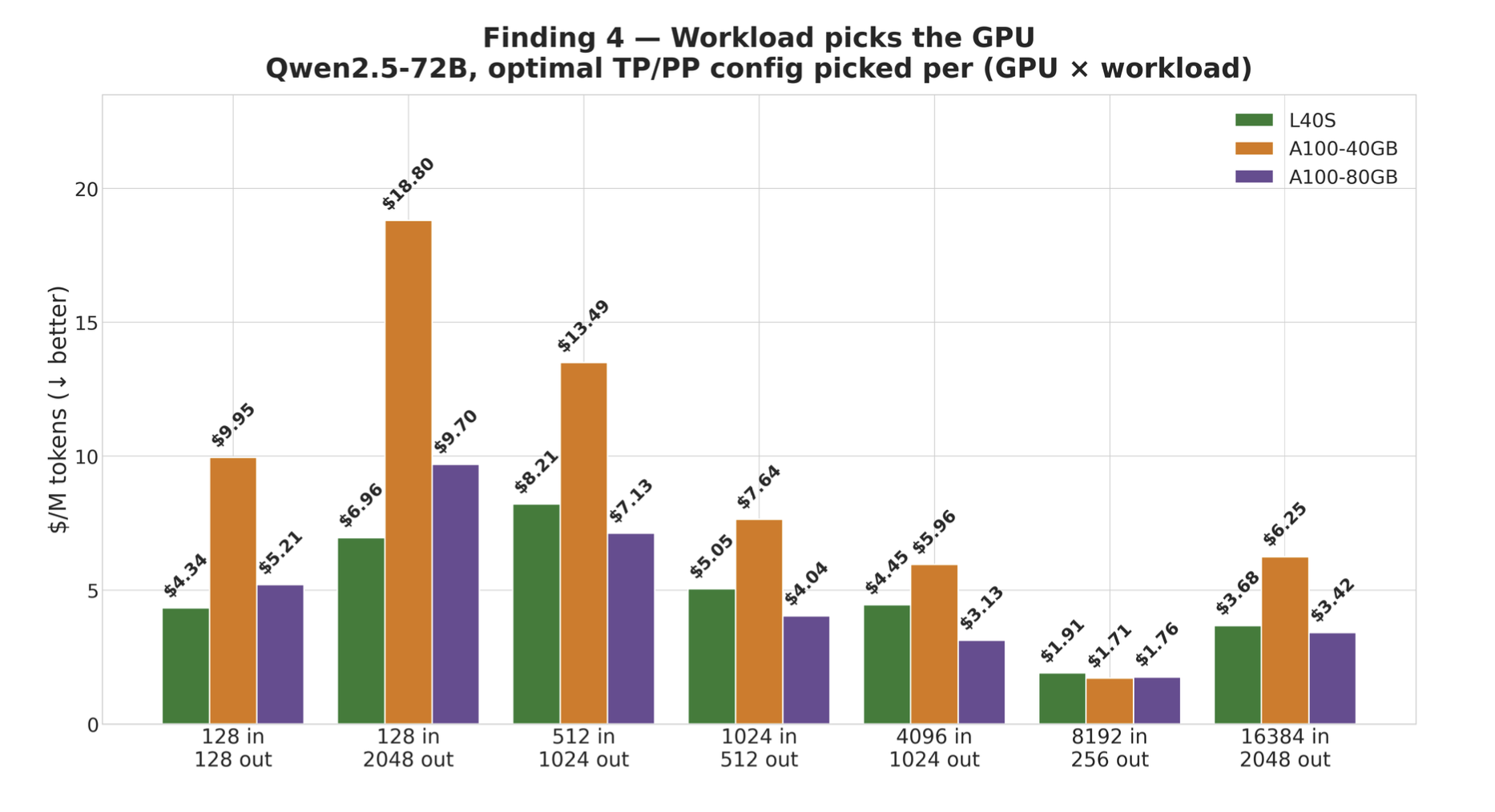 Figure 4. Best achievable $/M tokens for Qwen2.5-72B across seven input/output token-length combinations on A100-80GB, L40S, and A100-40GB. For each (GPU × workload) cell the cost-optimal TP/PP configuration is picked. Same model, same engine.
Three things to read off this chart.
The cost floor moves 3-5× across workload shapes on every GPU. On L40S the cheapest workload (8192/256, RAG-like) costs $1.91/M tokens and the most expensive (512/1024, decode-leaning) costs $8.21/M — a 4.3× spread. On A100-80GB the same span is $1.76 → $9.70 = 5.5×. On A100-40GB, $1.71 → $18.80 = 11×. Workload shape is a first-class cost variable, not a knob the engine smooths over.
The cost-optimal GPU is workload-dependent. A100-80GB wins on 5 of 7 workloads, including the balanced and prefill-leaning ones. But L40S wins on 128/128 (autocomplete) and 128/2048 (decode-heavy chat), where the small prefill doesn't pay back A100-80GB's bandwidth advantage. A100-40GB never wins. There is no single "best GPU for Qwen2.5-72B" — the answer depends on what your users type.
Two products at your company built on the same 72B model on the same cluster can have 4-5× different unit economics depending only on what users do with them. A RAG product that retrieves 8k tokens and answers in 256 is fundamentally cheap to serve. A chatbot that takes a one-line question and writes a two-thousand-token essay is fundamentally expensive. The model and the hardware do not change this. Engine tuning does not close the gap. If you priced both products on the same per-token margin, one of them is leaving money on the table and the other one is losing money on every request.
Finding 5 — Decode taxes bigger models harder
Same hardware (L40S), same engine. Compare a 32B-parameter dense model (Qwen3-32B) with a 70-72B dense model (Qwen2.5-72B-Instruct). Naive scaling: 2.2× more parameters, expect ~2.2× higher $/M tokens. Reality is messier — the ratio varies from 1.5× to 3.7× depending on workload shape.
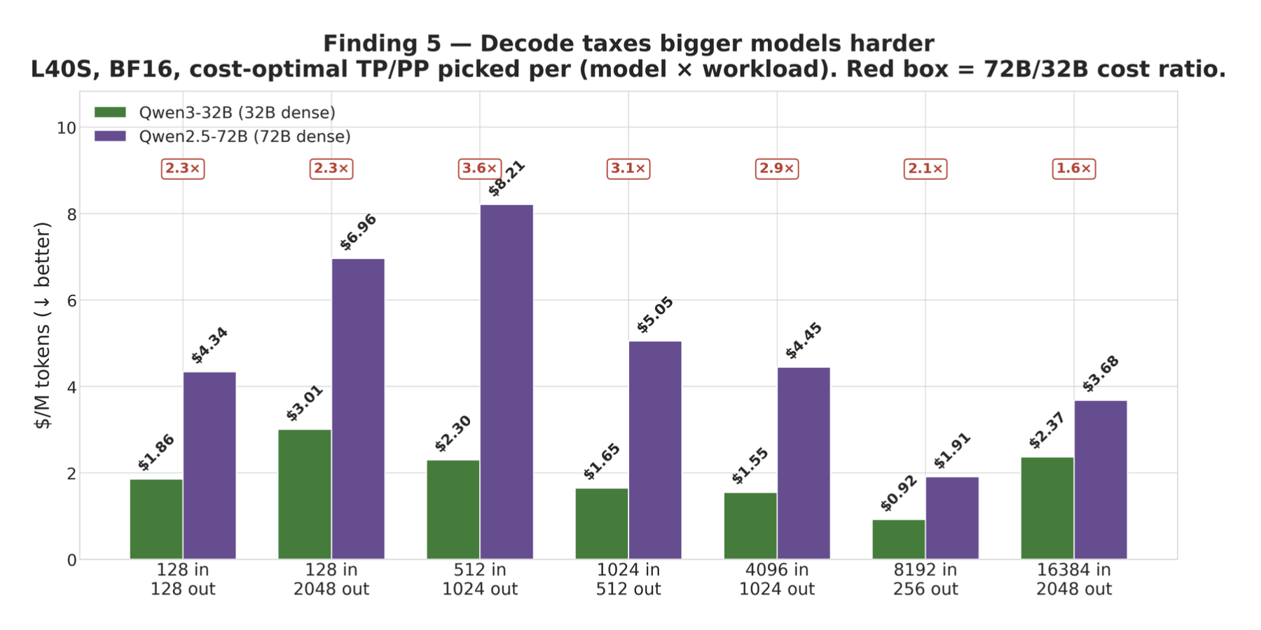 Figure 5. Best achievable $/M tokens for Qwen3-32B (32B dense) and Qwen2.5-72B-Instruct (72B dense) on L40S across seven input/output token-length combinations. Cost-optimal TP/PP picked per (model × workload).
Two things to read.
The cost ratio moves by 2.4×. On long-context (16384in / 2048out), the 72B model is only 1.5× more expensive per token than the 32B model — much less than the 2.2× parameter ratio. On decode-heavy (512in / 1024out), the 72B is 3.6× more expensive — far more than the parameter ratio. Decode is pure weight streaming, so per-token cost scales with weight bytes streamed per GPU, which is bigger and more concentrated for the 72B; the bigger model gets disproportionately punished. Prefill amortizes the same weight streaming over many tokens, so the disadvantage shrinks.
The optimal config changes too. Qwen3-32B wins 5/7 workloads with TP=4 PP=4. Qwen2.5-72B wins 5/7 workloads with TP=4 PP=2 or PP=3. Same family of GPU, same engine, just a 2.2× parameter ratio — and the right parallelism setting shifts. A rule tuned on 70B does not survive a 32B sweep; it doesn't even survive a 72B sweep at every workload shape.
MoE models like Qwen3-235B-A22B don't follow this pattern at all — the cost-optimal config depends on sparse-activation physics that dense scaling rules don't capture. Part 5.
Finding 6 — The premium GPU isn't proportionally cheaper
I want to revise something I said in ep2.
If you look at the cheapest $/M for 70B on each GPU, L40S wins comfortably over A10G — ep2 explained that as "70B can't fit in 4× A10G, so A10G is forced into bad configs." That framing was correct as far as it went. The story gets sharper when you bring A100 into the picture.
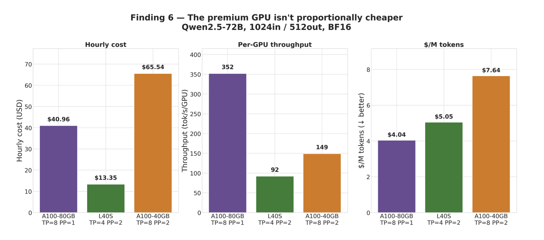 Figure 6. Three GPUs side by side on the same workload (Qwen2.5-72B, 1024/512, BF16) at their best $/M configuration. Left: hourly cost (A100-80GB is 3.07× L40S; A100-40GB is 4.91× L40S because it needs 2 nodes to fit comfortably). Middle: per-GPU throughput (A100-80GB ~3.8× L40S, A100-40GB ~1.6× L40S). Right: $/M tokens — A100-80GB ends up 20% cheaper than L40S; A100-40GB ends up 51% more expensive.
A100-80GB beats L40S, but by only 20%. A100-40GB loses to L40S, despite NVLink and higher HBM bandwidth and being marketed as the "professional inference" tier. Neither result is what the spec sheet predicts. The decomposition is worth showing because it tells you when the premium tier actually pays for itself and when it doesn't.
A100-80GB vs L40S — where the 20% comes from.
Hourly cost ratio: 40.96 / 13.35 = 3.07× more expensive
Throughput ratio: 2814 / 735 = 3.83× more throughput
$/M ratio: 3.07 / 3.83 = 0.80× → 20% cheaper per token
That 3.83× per-GPU throughput uplift breaks down into two clean pieces. First, HBM bandwidth: A100-80GB at 2039 GB/s vs L40S at 864 GB/s = 2.36×. That's the pure decode-bound roofline gain. Second, KV-cache headroom: after weights, A100-80GB leaves 50 GB/GPU available for KV cache; L40S leaves 22.8 GB/GPU. ~2.2× more KV space sustains roughly 2× larger concurrent batch, which improves attention arithmetic intensity by ~1.6×. The product (2.36 × 1.6 ≈ 3.8) matches the measured ratio. No magic. A100-80GB's bandwidth and VRAM both pay back; NVLink contributes essentially nothing at this workload because dense 72B at batch ~30 isn't communication-bound.
A100-40GB vs L40S — why the premium GPU loses.
Hourly cost ratio: 65.54 / 13.35 = 4.91× more expensive (forced into 2 nodes because TP=8 PP=1 single-node tops out at 996 tok/s, worse $/M than the 2-node config)
Throughput ratio: 2384 / 735 = 3.24× more throughput
$/M ratio: 4.91 / 3.24 = 1.51× → 51% more expensive per token
A100-40GB has 1.8× more HBM bandwidth than L40S and NVLink, but at dense 72B with moderate batch sizes the workload is not communication-limited and the KV cache headroom (smaller than A100-80GB's) doesn't pay back enough to justify the price. Most of the configurations where A100-40GB's premium features would activate are precisely the configurations where you would have just picked A100-80GB instead. A100-40GB sits in an awkward sweet spot of "expensive enough to be a premium tier, not high-VRAM enough to take advantage of it."
The real principle, restated cleanly: hardware that can host the model in the smallest TP group with meaningful KV-cache headroom wins on $/token. For 70-72B BF16, L40S is the cheapest GPU where TP=4 PP=2 fits comfortably and runs at decent batch. A100-80GB delivers 20% better $/M because the bandwidth gain + the bigger batch from 80 GB VRAM partially repay the 3× hourly premium. A100-40GB delivers a worse $/M than L40S because it costs almost as much as A100-80GB but cannot host larger batches and gets stuck in cross-node configs.
You cannot pick a GPU once and reuse the choice across model sizes or workload shapes. Each model has its own "smallest GPU where the cheap config is even legal" — and that is what you want.
The takeaway
Dense LLM serving cost is a 6-dimensional optimization problem (model × workload × GPU × parallelism × engine × topology), and the dimensions are not separable. No spec sheet, rule, or single-axis dashboard recovers the cost-optimal config. Picking blindly costs 2-5× on $/M tokens.
Three things to do tomorrow:
-
Optimize $/M tokens directly. SM% and HBM% can both be 99% on the worst-cost config. The cheapest honest dashboard proxy is tok/s/GPU — when it drops below half what you saw on a smaller config, your marginal GPUs are dead weight.
-
Don't reuse a config across workload shapes. Same model, same hardware: 8192in/256out is 4× cheaper per token than 512in/1024out. The cost-optimal config for RAG is rarely the cost-optimal config for chat. If you serve both off one pool, one is silently subsidizing the other.
-
Don't pick a GPU once. A100-80GB wins most workloads; L40S wins on short prompts and decode-heavy chat; A100-40GB almost never wins. The right GPU shifts with model size and workload shape, not with the spec sheet.
Why the standard tools cannot settle this
Every observation above is outside what off-the-shelf analysis predicts: roofline models miss engine scheduler overhead, KV pressure, NCCL contention and pipeline-bubble amortization (and overestimate throughput by 30–60% in our data); operator-level simulators (Vidur) re-introduce a profiling cost specific to each GPU/driver/kernel version; black-box config selectors (CherryPick, Ernest) assume smooth low-dimensional surfaces while our feasible set is riddled with binary cliffs (head divisibility, VRAM, NCCL compatibility); training-stack parallelism compilers (Alpa, Pollux, Tiresias) solve a different problem with a different feedback signal; serving engines (vLLM, SGLang, TRT-LLM, Dynamo) optimize within a chosen TP/PP/GPU and treat that choice as input; multi-cloud orchestrators (SkyPilot, SkyServe) pick where to run, not what to run. Each captures a slice; none captures the joint, and the joint is where the cost lives.
Why this is structurally hard, not just annoying
Three properties stack: (1) T(c) has no closed form — the binding bottleneck shifts between compute, HBM bandwidth, KV cache, and collective communication as a function of both config and workload, and no single-layer model tracks the shift (Findings 2, 3, 5 are all this); (2) every evaluation is expensive and slow — provisioning + weights download + warm-up + sustained load is $5–40 and 10–30 minutes per config, ~15–20 GPU-hours for a full sweep on one model, which is why most teams measure once and never repeat; (3) T(c) drifts — engine major versions, NVIDIA driver updates, AWS host-generation swaps, and NCCL default-algorithm changes each shift T(c) by 10–30% on configs that were previously optimal, so any benchmark older than a few months is not an oracle about today. A one-shot benchmark, a static rule, and a simulator all fail under one of these three. The honest shape of the problem is an optimization that runs continuously, learns from every production deployment it sees, and corrects itself as the substrate moves.
That is what we are building at Tandemn.
Part 4 — NCCL, hardware topology, NUMA, and PCIe virtualization in the cloud. Why single-node TP=8 stalls at 99% SM, why cross-node beats single-node on $/token, all from the same root: virtualization hides the dual-socket / dual-root-complex layout, NCCL pins proxy threads on the wrong NUMA, all-reduce traffic crosses the inter-socket bus.
Part 5 — MoE serving: expert parallelism, expert-routing all-to-all, sparse activation, small-GEMM kernel tail. None of the dense-70B rules survive.
Stay tuned!
Copy status