Evidence-guided planning for the whole fleet

The planning algorithm jointly chooses how inference workloads are configured and where they run across a heterogeneous GPU fleet. It combines a persistent causal model of serving behavior, a hierarchy of planning agents, and deterministic prediction, scoring, and feasibility checks.

The novelty is how these pieces work together. Deployment evidence shapes the configurations agents propose. Deterministic tools evaluate those proposals. A shared selector assembles a feasible plan across jobs competing for the same capacity. Each deployment then updates the evidence used in the next planning cycle.

This connects model-level tuning to fleet-level allocation: the planning algorithm can find a better configuration for one workload while accounting for the resources and serving objectives of every other job.

\Phi(P)=\sum_{(i,L_i)\in P}\left[J_i(L_i)-\gamma p_i^{\mathrm{brk}}(L_i)-\lambda_t\mathrm{Switch}_i(L_i^{(t-1)},L_i)\right]+\beta_t\mathrm{Expl}(P)

The cluster score combines per-job serving value, subtracts serving risk and reconfiguration cost, and rewards deployments that improve the algorithm’s understanding of inference behavior.

The unit of optimization is the cluster plan

A deployment configuration determines GPU type, tensor and pipeline parallelism, replica counts, and runtime settings. Placement binds that configuration to actual capacity in a cluster, cloud, or region. These choices are coupled: a fast configuration for one job can consume hardware that another job has no alternative to.

The planning algorithm takes a snapshot of available resources and all active and pending jobs. It considers the fleet as one optimization pool while retaining each environment’s hardware and performance characteristics. The resulting plan assigns a deployment to each job, retains an existing deployment, or defers admission when suitable capacity is unavailable.

For example, a job with several viable GPU options can use an alternative configuration, leaving a scarce accelerator for a workload that needs it. The planner evaluates that choice as part of the full allocation, rather than committing to each job’s preferred hardware independently. This is how configuration search can unlock additional usable capacity without changing the fleet.

The DAG connects decisions to serving behavior

The planning algorithm represents inference behavior as a directed acyclic graph, or DAG, with a fixed structure: deployment decisions affect runtime mechanisms, which affect serving outcomes. The graph follows the path X → V → Y.

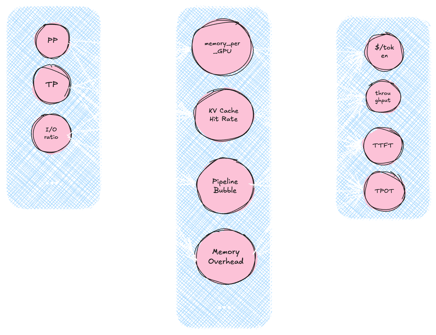
The causal DAG links parallelism and workload decisions to memory use, KV-cache hit rate, and pipeline behavior, then to token cost, throughput, TTFT, and TPOT. — Read the graph from left to right: deployment choices, such as pipeline parallelism (PP) and tensor parallelism (TP), affect runtime behavior, including memory use, KV-cache hit rate, and pipeline idle time. These mechanisms influence token cost, throughput, time to first token (TTFT), and time per output token (TPOT). The planning algorithm uses these relationships to trace performance bottlenecks back to configuration choices and updates its confidence in them as deployments produce new evidence.

This structure helps distinguish causes that can produce similar symptoms. Poor throughput caused by KV-cache pressure may need a different intervention from poor throughput caused by communication overhead. The graph lets agents trace a serving objective back to the deployment decisions and mechanisms that influence it.

Related edges form scoped hypotheses, called mechanisms, that apply to particular models, hardware, workloads, and conditions. Each relationship carries confidence and uncertainty. The planning algorithm compares predicted runtime behavior and serving outcomes with observations, then updates that evidence. Learning persists across planning cycles; the graph’s registered edges stay fixed while confidence and scoped hypotheses evolve.

Each job has its own objectives and score

A candidate deployment is evaluated against the workload it will actually serve. The planning algorithm uses operator-level latency profiles and a replay simulator to predict serving performance, then derives cost and objective attainment from the allocation and the job’s targets.

Serving objectives
Metric	Measure	Target
TTFT	First-token latency · p99	Lower
TPOT	Output-token latency · p99	Lower
Throughput	Tokens per second	Higher
Cost per token	Allocation cost / token	Lower
SLO margin	Headroom to serving target	Higher

Each job supplies weights expressing the relative importance of these objectives. An interactive service can emphasize TTFT and TPOT, while a batch workload can emphasize throughput and cost subject to its completion deadline. Serving requirements remain constraints on which deployments are eligible.

The planning algorithm normalizes each predicted outcome against a job-specific reference and combines the weighted gaps into an augmented Tchebycheff score. Its main term penalizes the largest weighted gap, so a strong result on one metric does not hide a weak result on another weighted objective. A smaller sum term distinguishes candidates with the same largest gap.

These objective weights describe how a job should run. Scheduling priority and capacity quotas separately govern how jobs compete for shared resources. The planner evaluates the objectives together, making improvements across several dimensions visible in the same score.

Mathematical formulation

Causal evidence

X\rightarrow V\rightarrow Y,\qquad p_e\sim\mathrm{Beta}(\alpha_e,\beta_e)

Decisions X affect runtime mediators V, which affect serving outcomes Y. Each graph edge carries a belief updated from supporting and contradictory deployment evidence. Its confidence and normalized uncertainty are:

c_e=\frac{\alpha_e}{\alpha_e+\beta_e},\qquad U_e=\frac{12\alpha_e\beta_e}{(\alpha_e+\beta_e)^2(\alpha_e+\beta_e+1)}

Scoped mechanisms group these relationships into testable hypotheses. Confidence guides future proposals; uncertainty helps identify informative deployments to explore.

Job outcomes and priorities

Let $L_i$ be job i’s deployment ladder: the set of configurations, environments, and replica groups assigned to it. Its predicted outcome vector and objective weights are:

\mathbf y_i(L_i)=\bigl(\text{cost/token},\text{p99 TTFT},\text{p99 TPOT},\text{throughput},\text{SLO margin}\bigr)

w_{ij}\ge0,\qquad \sum_j w_{ij}=1

Cost, TTFT, and TPOT are minimized; throughput and SLO margin are maximized. The planning algorithm normalizes each outcome against a job-specific ideal reference $z_{ij}^{\star}$ using scale $\sigma_{ij}$ :

g_{ij}(L_i)=\begin{cases}\bigl(y_{ij}(L_i)-z_{ij}^{\star}\bigr)/\sigma_{ij},&\text{metric minimized},\\\bigl(z_{ij}^{\star}-y_{ij}(L_i)\bigr)/\sigma_{ij},&\text{metric maximized}.\end{cases}

The augmented Tchebycheff job score is:

J_i(L_i)=-\left[\max_j w_{ij}g_{ij}(L_i)+\rho\sum_j w_{ij}g_{ij}(L_i)\right]

The largest weighted gap drives the score. The sum term, weighted by $\rho$ , distinguishes candidates with the same maximum gap. Higher scores indicate closer alignment with the job’s weighted objectives.

Learning value, serving risk, and switching cost

Exploration rewards testing uncertain edges and mechanisms. Activation indicators count whether any deployment in the plan tests a relationship:

\mathrm{Expl}(P)=\sum_{e\in E}A_e(P)U_e+\omega_m\sum_{m\in\mathcal M}A_m(P)U_m

$A_e(P)$ and $A_m(P)$ activate each edge or mechanism once per plan. $\omega_m$ weights mechanism uncertainty separately from edge uncertainty.

Breach estimates come from prediction-error bands calibrated against observed residuals. Per-objective estimates are combined using the implementation’s independence approximation:

p_i^{\mathrm{brk}}(L_i)=1-\prod_{j\in\mathcal S_i}\left(1-p_j^{\mathrm{brk}}\right)

$\mathcal S_i$ contains the job’s constrained serving objectives. Changing a running deployment also incurs:

\mathrm{Switch}_i=C_{\mathrm{cold}}+C_{\mathrm{parallel}}+C_{\mathrm{kill}}+C_{\mathrm{risk}}

These terms account for loading and warm-up, concurrent execution, draining and termination, and transient underperformance. They are zero when the deployment is retained.

Cluster objective and selection

A plan $P=\{L_i\}$ assigns a ladder to every active and pending job. Retaining the previous ladder keeps an active deployment; an empty ladder defers a pending job. The cluster score is:

\Phi(P)=\sum_{(i,L_i)\in P}\left[J_i(L_i)-\gamma p_i^{\mathrm{brk}}(L_i)-\lambda_t\mathrm{Switch}_i(L_i^{(t-1)},L_i)\right]+\beta_t\mathrm{Expl}(P)

$\gamma$ weights serving risk, $\lambda_t$ weights reconfiguration cost, and $\beta_t$ weights learning value. Exploration and switching weights adapt across planning cycles.

The optimization goal is:

P_t\in\arg\max_{P\in\mathcal F_t}\Phi(P)

$\mathcal F_t$ contains plans satisfying resource capacity, physical deployment, serving-risk, active-swap-budget, quota, and priority constraints. Search is bounded, so the planning algorithm commits the highest-scoring feasible plan it finds rather than an exhaustive global optimum. New telemetry updates the evidence for the next cycle.

Read the research behind the formulation

Before you buy more GPUs, see what your fleet can do.

Show us your workloads and serving stack. We’ll walk through how Tandemn can unlock more capacity from the hardware you already have.

Schedule a demo